
Carbon emissions of ocean freight: what is your value at risk?
When looking to invest your savings in a portfolio, you are likely to scout for asset managers with good past performance. It is natural to seek reassurance by examining the history of the returns of a fund. Most often than not, it’s even in the brochure: “Our alpha lambda fund has shown an average past performance of 5.6% per year over the last 10 years”. Should you invest?
On the fallacy of averages.
As a seasoned investor, you know the fallacy of averages. On average, a drunk man will walk in a straight line, right in the middle of the road, with cars driving left and right. On average, the drunk man is alive. In real life however, his walk will take him left and right, randomly. Almost surely, he will hit a car on either side, and die.
There is no doubting our ability to make wise investment decisions. And, admittedly, the portfolio allocation problem has somewhat been solved today, with a panoply of tools allowing one to make the right choice, factoring in value at risk, volatility, max drawdown, and other metrics.
That’s for investment strategy. In the world of logistics, when talking carbon reduction strategy, why is it that we still rely on averages in 2022?
Carbon emissions of ocean freight.
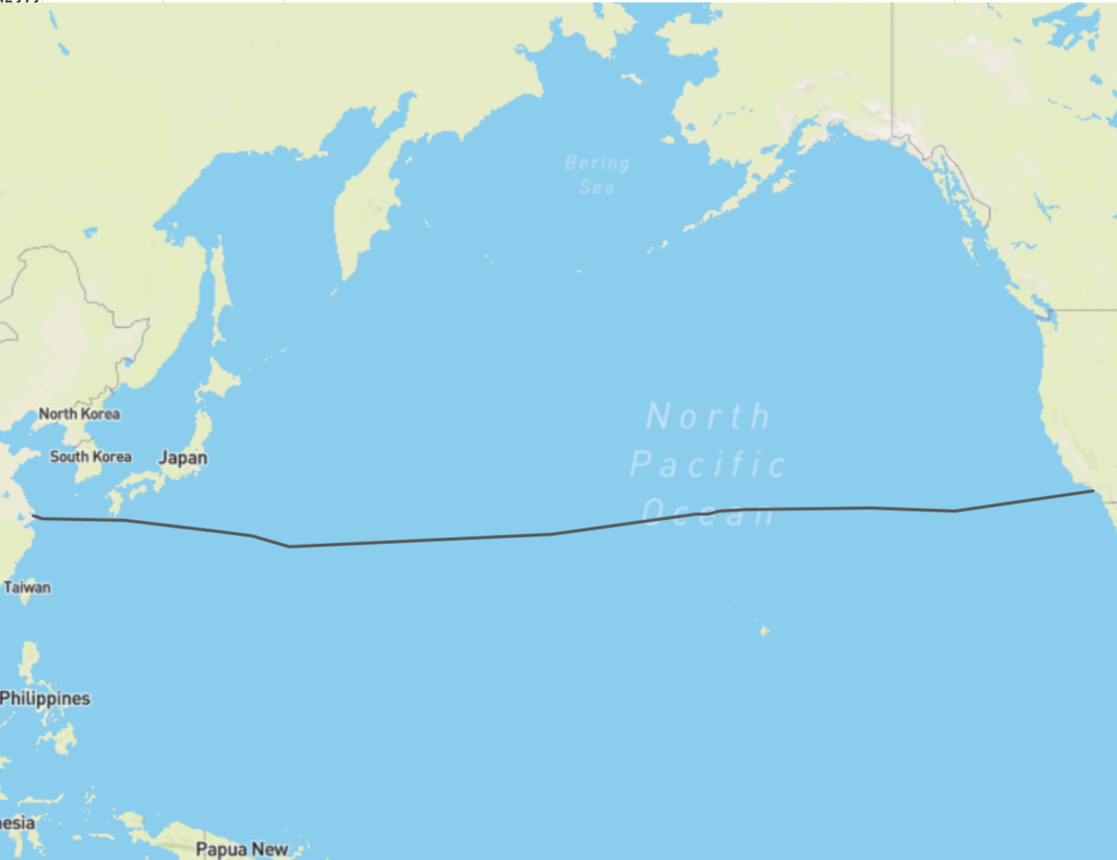
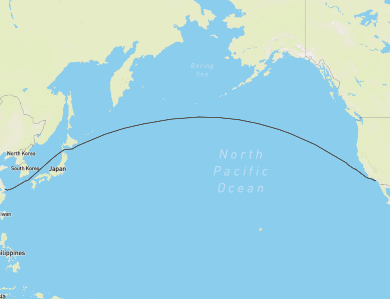
For the purpose of illustration, let’s consider a transpacific trade, between Shanghai (CNSHA) and Los Angeles (USLAX). We are seeking to estimate the CO2 emissions of one twenty-foot equivalent (TEU) container, the standard unit of measurement of ocean freight.
The Global Logistics Emission Council (GLEC) has designed a framework which unifies methodologies to estimate carbon emissions of all transport modes. For ocean freight, the methodology follows the recommendations of the Clean Cargo Working Group (CCWG), which provides emission factors per trade lane (publicly) and per carrier (for CCWG members). This methodology provides a good baseline for our estimations. From the GLEC methodology document, one can read:
| Tradelane | Container type | Aggregate average trade lane emission factor, in g CO2/TEU -km |
|---|---|---|
| Asia to-from North America WC | Dry | 67.1 |
| Reefer | 116.5 |
With these numbers in mind, the CO2 emissions of 1 TEU is 1 TEU x Tradelane Emission Factor x Distance (CNSHA – USLAX) = 0.69 tons CO2. In this simple equation, only the distance is an adjustable parameter. It is commonly accepted that one should use the shortest sailable distance, adjusted by 15% [see GLEC]. But we already see how this will be problematic.
Difficult to make an investment decision based on averages. Difficult to make an allocation decision based on averages.
Someone working in procurement, at a large retail company, may find himself stuck with this one number: 0.69 tons of CO2 between Shanghai and Los Angeles, whatever the vessel, whatever the sequence of port calls, whatever the fleet or the carrier.
Difficult to make an allocation decision based on averages!
The physics of ocean freight as the better estimator.
If we look closer at the physics of ocean freight, carriers operate fleets of vessels of different sizes and ages, they form alliances around a particular sequence of port calls (called a service), on which the speed and distance sailed vary. Because of this reality, the CO2 of a portfolio of ocean freight, just like the return of a portfolio of stocks, shows value at risk, volatility, max drawdown, and other metrics.
When moving away from averages, and estimating the CO2 emissions of every vessel assigned to a service sailing the Asia to-from North America WC trade lane, the picture looks like this:
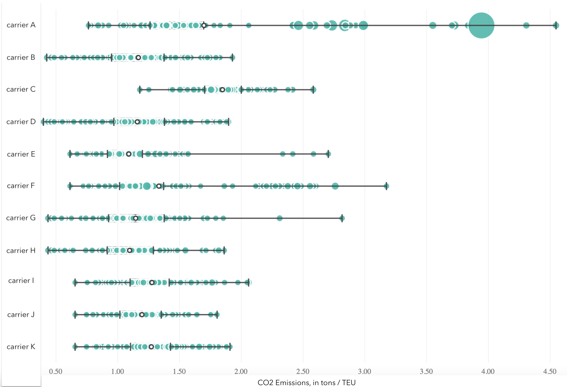
In this picture, each green bubble represents a service operated by a carrier and its alliance, between an Asian port and a North America west coast port. The bubble is placed horizontally on the x-axis depending on the average CO2 of that service. The radius of the bubble shows the volatility in carbon emissions of that service. The more inhomogeneous the fleet of a particular service (and its alliance), the larger the bubble.
Just as in the case of the random walk of the drunk man, what is striking on that picture is the spread of values. The conclusion of our modelling is that the carbon emissions reported by carriers are likely to fluctuate left and right. The amplitude of these fluctuations, and the baseline average is specific to each carrier and its alliance. The good news: there is a lot of room to allocate wisely!
For our specific port pair, Shanghai to Los Angeles, we can look at the specifics of 5 services operated by the 3 largest ocean alliances. We report in the table below the CO2 emissions averaged across the vessels operating each service. Which service would you pick to reduce your carbon emission bill?
| co2 avg | co2 min | co2 max | co2 std | intensity | service names |
|---|---|---|---|---|---|
| 1.05 | 0.88 | 1.18 | 0.09 | 0.96 | Alliance Service A |
| 0.61 | 0.38 | 0.86 | 0.14 | 0.57 | Alliance Service B |
| 1.16 | 0.91 | 1.40 | 0.13 | 1.09 | Alliance Service C |
| 0.82 | 0.75 | 0.98 | 0.07 | 0.75 | Alliance Service D |
| 1.06 | 0.99 | 1.16 | 0.07 | 0.99 | Alliance Service E |
We notice that the service with the lowest average CO2 values (Service B) is also the most volatile. This means the fleet on this service is heterogeneous in size and age. As comparable transit time and rates, we’d most likely choose service D, which has the best risk / return ratio, as see on the graph below.

The physics of ocean freight shows us there are many more colours to the rainbow than a single average. Like in the case of an investment decision, carbon emissions management starts with an understanding of the right metrics of volatility and risk.
The question remains however, if Searoutes model is a better estimator of the future (than one average value), is the past an even better predictor?
Is the past a good estimator of the future?
To continue our portfolio management analogy, returns and volatility cannot only be based on models. Models are useful to estimate the future, but only the raw data will paint the right picture of the past.
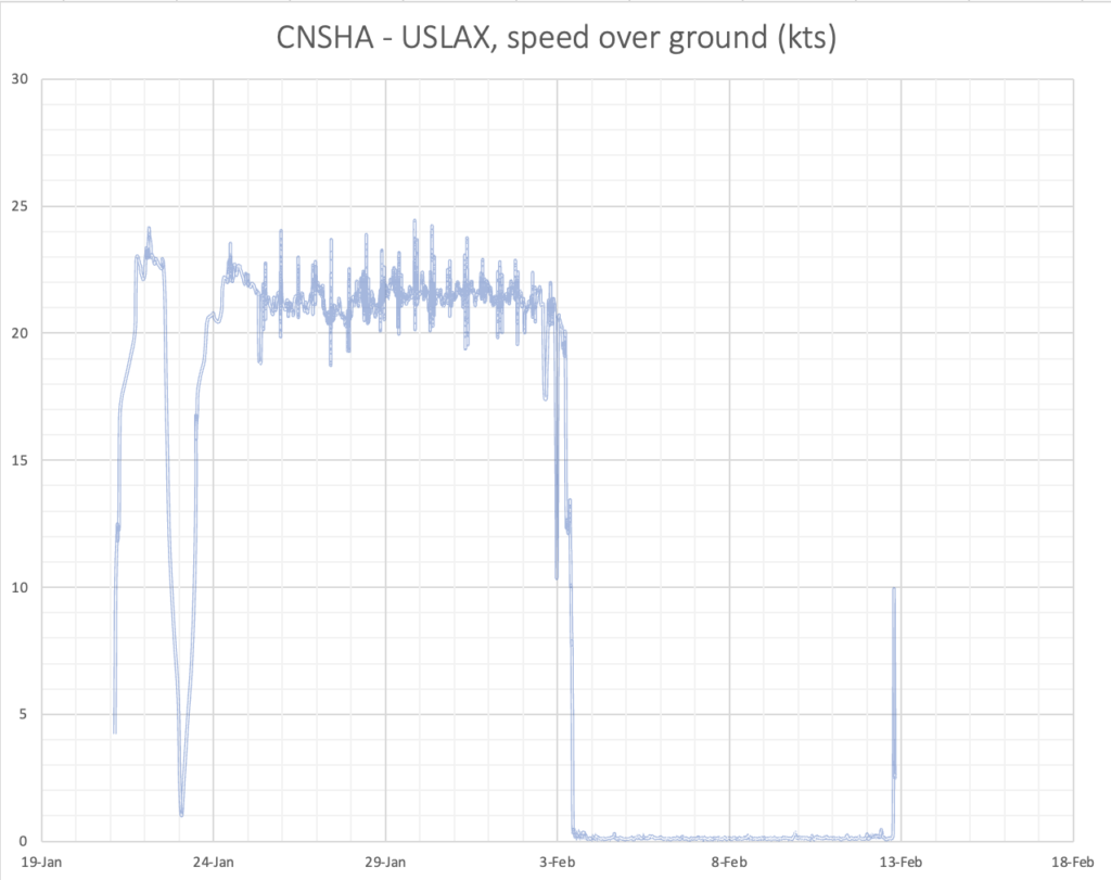
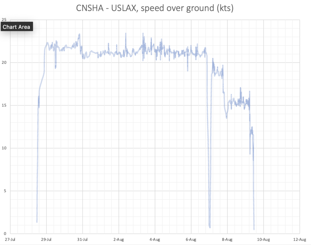
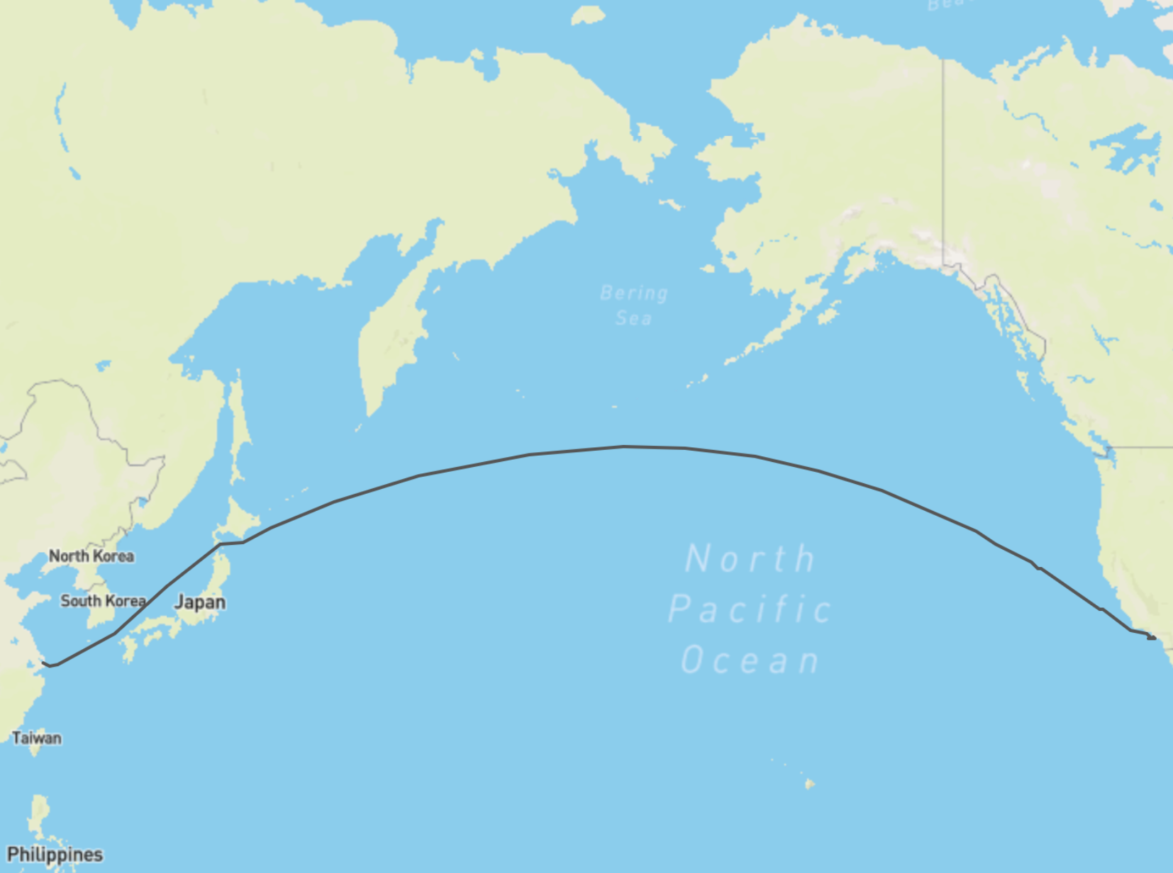
Luckily, data is not a scarce commodity in ocean freight. The AIS revolution has given us the position and the speed of every vessel worldwide, and this comes in handy for our CO2 estimation story. Not unexpectedly, raw data shows a wide variation in distances, and speeds. We plot 3 trajectories of the same vessel, at 3 different time periods.
January 21
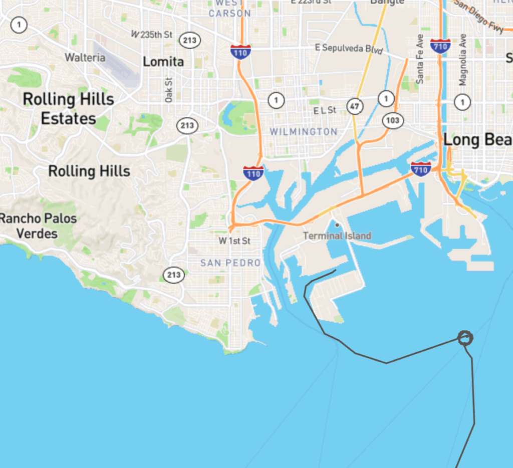
July 21
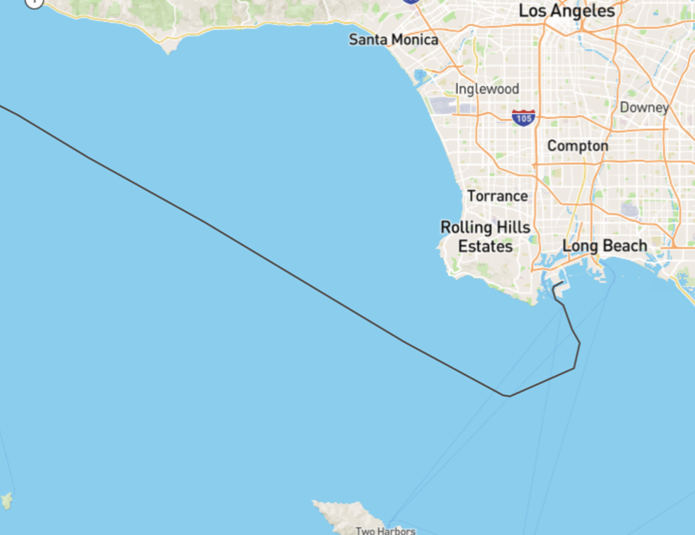
September 21
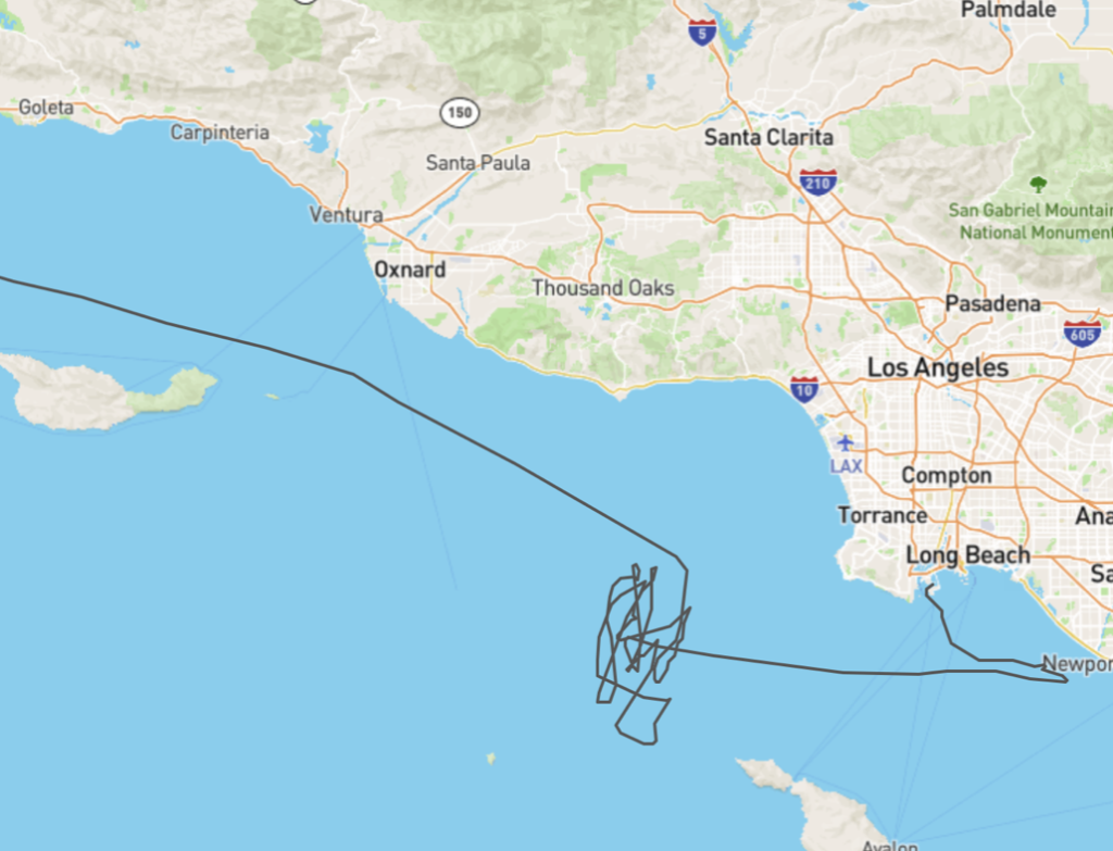
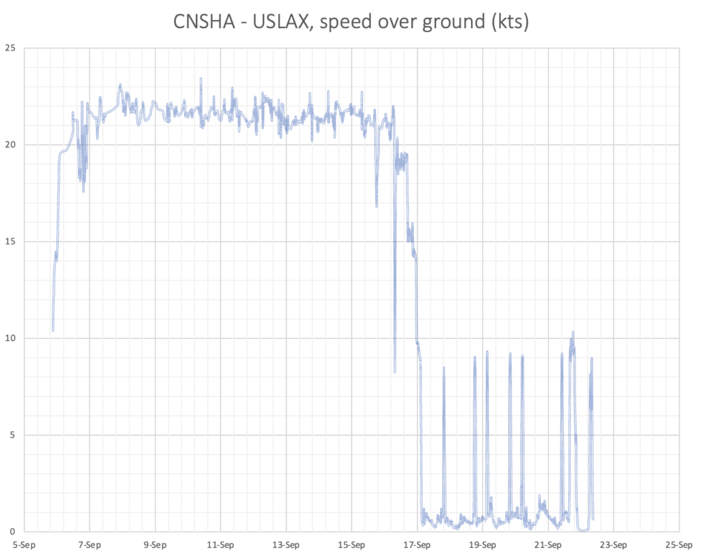
Focusing on the real trajectories of vessels, we can compute the actual emissions of Service C below.
| Vessel imo | co2 min | co2 max | co2 average | co2 std |
|---|---|---|---|---|
| 9xxxxx1 | 1.81 | 2.01 | 1.88 | 0.07 |
| 9xxxxx2 | 1.61 | 1.78 | 1.70 | 0.09 |
| 9xxxxx3 | 1.65 | 1.98 | 1.81 | 0.10 |
| 9xxxxx4 | 1.82 | 1.96 | 1.90 | 0.04 |
| 9xxxxx5 | 1.94 | 2.17 | 2.05 | 0.08 |
| 9xxxxx6 | 1.61 | 1.78 | 1.70 | 0.09 |
Conclusion
Managing carbon emissions in the logistics is a bit like portfolio management. One cannot realistically make good choices solely based on averages. Ocean freight has inherent physics which creates spreads and volatility in carbon emissions. The right model helps frame and estimate these, so the right objectives, and subsequent reduction strategy is put in place. Just like in finance, past data points can be used to better calibrate our models. And, just like with your 401k, your long term trend will converge to your goals.
Let us know if you would be interested in getting detailed carbon emissions data or to further explore your entire logistics footprint and gain control of your logistics carbon emissions today!
Carbon Footprint, CO2 calculation, CO2 emissions, Green shipping, Sustainability